Spatial Smoothing with the Network Lasso#

This guide walks through a small-area-estimation problem: we have noisy per-county survey estimates of (log) median household income across the state of Georgia and we want a smoothed map that borrows strength between neighboring counties. The natural tool is gamdist’s categorical feature with network lasso regularization on the county-adjacency graph, which adds an L1 penalty to coefficient differences along graph edges and therefore fuses neighbors to identical values rather than merely shrinking them toward each other.

By the end you will have produced a three-panel choropleth contrasting the raw observations, the network-lasso fit, and the (simulated) ground truth, and you will have seen how to obtain real county geometries with a couple of lines of geopandas — no hand-curated SVG required.

Extra dependencies#

The example uses two libraries that are not runtime dependencies of gamdist itself:

geopandas for reading the county shapefile and rendering the choropleth.
libpysal for the bundled Georgia counties dataset and for building the Queen-contiguity adjacency graph.

Install them into your environment alongside gamdist:

pip install geopandas libpysal

The same workflow generalizes to any other shapefile or GeoJSON of geographic units — US counties from the Census TIGER/Line files, ZIP-code tabulation areas, school districts, electoral precincts, and so on. We use Georgia’s 159 counties because the geometries are bundled with libpysal and the example runs in a few seconds.

Loading the geometry#

libpysal.examples ships a small library of spatial datasets that load without an internet round-trip. The georgia example contains a shapefile of Georgia’s 159 counties together with 1990 socio-economic attributes. We need only the geometries:

import geopandas as gpd
from libpysal.examples import load_example

ex = load_example('georgia')
counties = gpd.read_file(ex.get_path('G_utm.shp'))
counties['county_id'] = counties['AreaKey'].astype(str)

print(counties.shape)         # (159, 18)
print(sorted(counties.columns)[:6])
# ['AREA', 'AreaKey', 'G_UTM_', 'G_UTM_ID', 'Latitude', 'Longitud']

A geopandas.GeoDataFrame is a regular pandas.DataFrame with one extra column — geometry — holding a Shapely polygon per row. AreaKey is the FIPS code; we promote it to a string so it can serve as our categorical level.

Building the adjacency graph#

Network lasso needs an edge list: a DataFrame with three columns node1, node2, and weight describing which categories should be encouraged to share a coefficient. For spatial data the natural choice is Queen contiguity: two polygons are neighbors if they share any boundary point (vertex or edge). libpysal.weights has this built in:

import pandas as pd
from libpysal.weights import Queen

w = Queen.from_dataframe(counties, use_index=False)

pairs = []
for i, neighbors in w.neighbors.items():
    for j in neighbors:
        if i < j:                       # each undirected edge once
            pairs.append((counties.iloc[i]['county_id'],
                          counties.iloc[j]['county_id']))
edges = pd.DataFrame(pairs, columns=['node1', 'node2'])
edges['weight'] = 1.0

print(len(edges))    # 431

Each row of edges says “these two counties are neighbors and should contribute a penalty term weight * |β_node1 - β_node2| to the fit”. A larger weight makes the corresponding pair more strongly fused; uniform 1.0 weights are the typical starting point. Use Rook.from_dataframe instead if you want only edge-sharing neighbors (i.e., excluding pairs that meet at a single corner).

Simulating the response#

To demonstrate the smoother we’ll synthesize a smooth-along-the-graph truth and corrupt it with sampling noise. The true log-income declines radially from a peak near metro Atlanta:

import numpy as np

rng = np.random.default_rng(0)
atlanta_lat, atlanta_lon = 33.75, -84.39
dist_to_atl = np.sqrt(
    (counties['Latitude'] - atlanta_lat) ** 2
    + (counties['Longitud'] - atlanta_lon) ** 2
)
counties['true_log_income'] = 10.8 - 0.25 * dist_to_atl

We then draw five noisy observations per county, as if from a survey with five respondents in each:

obs_rows = []
for _, row in counties.iterrows():
    for _ in range(5):
        obs_rows.append({
            'county_id': row['county_id'],
            'log_income': row['true_log_income'] + rng.normal(0, 0.30),
        })
obs = pd.DataFrame(obs_rows)
print(len(obs))   # 795

The unsmoothed estimate for each county is just the per-county sample mean:

counties['observed_mean'] = (
    counties['county_id']
    .map(obs.groupby('county_id')['log_income'].mean())
)

Fitting the GAM#

The model has a single feature — county_id, treated as a categorical with network-lasso regularization. The regularization dict pairs the coefficient \(\lambda\) with the edge list. We start from \(\lambda = 0.25\), which a moment of GCV-driven tuning (next section) will confirm is a good default for this dataset:

from gamdist import GAM

mdl = GAM(family='normal')
mdl.add_feature(
    name='county_id',
    type='categorical',
    regularization={'network_lasso': {'coef': 0.25, 'edges': edges}},
)
mdl.fit(obs[['county_id']], obs['log_income'].to_numpy())

mdl.summary()
# Model Statistics
# ----------------
# phi: 0.0890
# edof: 51
# Deviance: 66.2
# AIC: 848
# AICc: 855
# BIC: 1091
# R^2: 0.408
# GCV: 0.0951

The fitted county effects — one per category — are obtained by calling predict() with a one-row-per-county DataFrame:

counties['fitted_log_income'] = mdl.predict(counties[['county_id']])

The reported effective degrees of freedom (51) is much smaller than the 159 categories: the network lasso has fused most neighboring counties to identical coefficients, and edof reflects the actual number of distinct fitted values rather than the unconstrained category count. That correctly-shrunk edof is what allows the AIC, BIC, and GCV numbers above to be compared meaningfully across \(\lambda\) values.

Drawing the choropleth#

geopandas.GeoDataFrame.plot() colors each polygon by the value in a chosen column. We render the raw observations, the network-lasso fit, and the underlying truth side by side, sharing a color scale so the panels are directly comparable:

import matplotlib.pyplot as plt

fig, axes = plt.subplots(1, 3, figsize=(15, 5), constrained_layout=True)
cols = ['observed_mean', 'fitted_log_income', 'true_log_income']
titles = ['Observed (noisy survey mean)', 'Network-lasso fit', 'Truth']
vmin = counties[cols].min().min()
vmax = counties[cols].max().max()
for ax, col, title in zip(axes, cols, titles):
    counties.plot(column=col, cmap='viridis', vmin=vmin, vmax=vmax,
                  edgecolor='white', linewidth=0.2, ax=ax)
    ax.set_axis_off()
    ax.set_title(title)
fig.suptitle('Simulated log median household income, Georgia counties')
plt.show()

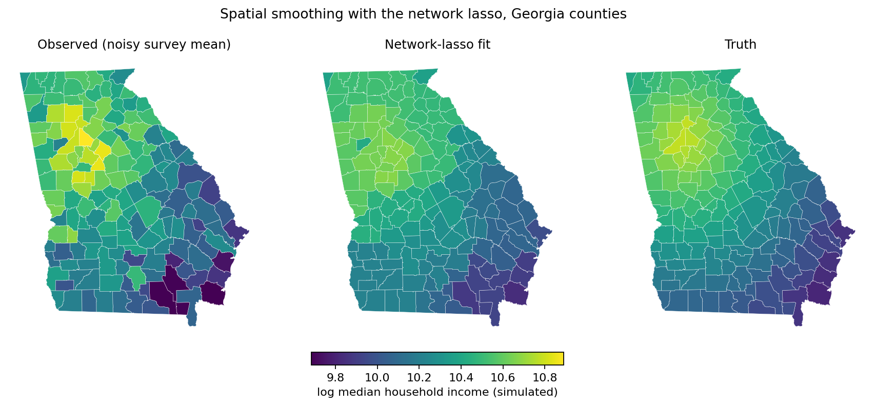
Three-panel choropleth of Georgia counties: noisy survey means on the left, the network-lasso fit in the middle, and the smooth truth on the right. — Network-lasso smoothing of a simulated per-county survey of log median household income at the GCV-optimal \(\lambda = 0.25\). The middle panel collapses 159 counties to 50 distinct fitted values; most internal boundaries disappear as neighbors fuse to identical coefficients.#

The left panel is mottled — noise dominates the per-county means. The middle panel shows the smoothed estimate: most county boundaries have vanished because the network lasso has fused neighboring counties to identical coefficients, leaving a small number of contiguous regions of constant value. The right panel is the smooth truth that the simulation drew from. Visually, the middle panel is much closer to the right than the left.

Choosing the smoothing strength#

The single tuning knob is \(\lambda\) (passed as coef). At \(\lambda = 0\) the categorical feature is unregularized and each county gets its own free coefficient (= the per-county sample mean, modulo the implicit zero-sum centering). As \(\lambda \to \infty\) all coefficients along any connected component of the graph collapse to the same value. The principled way to choose \(\lambda\) is to minimize generalized cross-validation (GCV), an efficient leave-one-out CV approximation reported by summary() on every fit:

for lam in [0.001, 0.05, 0.1, 0.25, 0.5, 1.0]:
    mdl_l = GAM(family='normal')
    mdl_l.add_feature(
        name='county_id', type='categorical',
        regularization={'network_lasso': {'coef': lam, 'edges': edges}},
    )
    mdl_l.fit(obs[['county_id']], obs['log_income'].to_numpy())
    fit = mdl_l.predict(counties[['county_id']])
    n_unique = np.unique(np.round(fit, 4)).size
    print(f'lambda={lam:>6}: edof={mdl_l.dof():>5.1f}'
          f'  GCV={mdl_l.gcv():.4f}  unique levels={n_unique:3d}')

# lambda= 0.001: edof=159.0  GCV=0.1146  unique levels=157
# lambda=  0.05: edof=124.0  GCV=0.1044  unique levels=123
# lambda=   0.1: edof=106.0  GCV=0.1020  unique levels=105
# lambda=  0.25: edof= 51.0  GCV=0.0951  unique levels= 50
# lambda=   0.5: edof= 34.0  GCV=0.0981  unique levels= 34
# lambda=   1.0: edof= 11.0  GCV=0.1009  unique levels= 11

GCV bottoms out near \(\lambda = 0.25\), where the network lasso has fused Georgia’s 159 counties into 50 contiguous regions of constant value. A negligible \(\lambda\) leaves nearly every county with its own value (157 distinct levels out of 159) and the fit barely improves on the raw per-county sample means. Push \(\lambda\) to 1.0 and the state is carved into 11 large regions: a clearer summary, but now over-smoothed where the truth is genuinely heterogeneous.

The edof column makes this concrete: it is the number of independent coefficients the fit is actually using, after fusion. For network_lasso dof() counts distinct fitted values rather than the unconstrained category count, so \(\lambda = 0.25\) and \(\lambda = 0.5\) both report edof that is far below 159 even though every county still has a (fused) prediction. That is what makes GCV — which weights the deviance by \((1 - \mathrm{edof}/n)^{-2}\) — a usable model-selection criterion here.

For a tighter optimum, sweep more \(\lambda\) values around the minimum and pick the one with the smallest GCV. Holding out part of the data and choosing \(\lambda\) by validation deviance gives the same answer up to noise, and is the standard fallback when you mistrust the GCV approximation (e.g., for very small samples or non-Gaussian families with a fixed dispersion).

When to reach for `network_lasso`#

Network lasso is the right tool when:

You have a categorical feature with a known graph structure (spatial adjacency, a hierarchy, a friend graph, related-products graph) and you believe many connected categories share a coefficient.
You want a piecewise-constant answer — a small number of homogeneous clusters — rather than a smoothly varying surface.

If you instead want smooth shrinkage along the graph (a quadratic penalty \(\lambda \sum_{(i,j) \in E} w_{ij} (\beta_i - \beta_j)^2\), which never collapses neighbors to identical values), swap network_lasso for network_ridge on the same edges DataFrame — the rest of the API is unchanged.