Evaluating Model Fit

A converged fit is not the same as a good fit. ADMM will happily return coefficients for a model whose family is wrong, whose link is mis-specified, or that is missing a feature with substantial predictive signal. This guide covers the two questions that come after fit() returns:

1. Is this model adequate? Does it describe the data, or does it leave systematic structure on the table?

2. Among candidate models, which should we prefer? When two fits both look reasonable, the right one is rarely the one with the smallest residual sum of squares.

The first question is answered by inspecting residuals; the second by information criteria. We work through both on the apartment-rent example from the Getting Started guide.

Before reading this guide, run the data-generation block from that guide to populate X and y; everything below assumes those names are in scope.

Information criteria

summary() reports six fit statistics:

• Deviance — twice the gap in log-likelihood between the fitted model and a saturated model that interpolates the data. Smaller is better, but adding any feature reduces deviance, so deviance alone is not a model-selection tool.

• R² — the deviance-based pseudo-\(R^2\), \(1 - D / D_0\), where \(D_0\) is the deviance of the intercept-only model. Same caveat: monotone in feature count.

• AIC (aic()) — deviance plus \(2 p\), where \(p\) is the effective parameter count. Penalizes complexity; lower is better; differences below 2 are usually not meaningful.

• AICc (aicc()) — AIC with the Hurvich-Tsai small-sample correction. Identical to AIC asymptotically; prefer it when \(n / p\) is small (rule of thumb: \(n / p < 40\)).

• BIC — deviance plus \(p \log n\). Penalizes complexity more aggressively than AIC and is consistent for selecting the true model when one exists in the candidate set.

• GCV (gcv()) / UBRE (ubre()) — generalized cross-validation and the unbiased risk estimator. Both approximate out-of-sample squared error without refitting. summary() prints UBRE when the family fixes the dispersion (Poisson, binomial) and GCV otherwise.

For routine model comparison, AIC (or AICc on small samples) is the most useful single number. Use BIC when you specifically want a parsimonious model and believe the true effect set is finite. Use GCV to choose the smoothing of a single spline at fixed model structure.

A worked comparison

The Getting Started guide fit three nested models on the rent data. Their fit statistics:

Model	edof	Deviance	AIC	AICc	R2
sqft only	2	67.1	504	504	0.79
neighborhood	5	14.6	507	507	0.95
walkability (spline)	9	5.4	511	511	0.98

Two things are worth noting. First, AIC increases with each addition even though deviance and \(R^2\) improve. AIC penalizes a feature by \(2 \hat\phi\) per effective degree of freedom, and as \(\hat\phi\) shrinks — which it does each time we explain more variance — the threshold a new feature must clear gets lower. The absolute AIC is not directly interpretable; only differences between models on the same data are. Second, the AIC differences here are small (3, then 4), so on AIC alone the case for mdl3 over mdl1 is suggestive rather than decisive. Residual diagnostics settle the question conclusively, as we will see below.

Residuals

For a Gaussian model with identity link, residuals are simply \(y - \hat{y}\). For other families, that definition is not useful: a Bernoulli observation is 0 or 1, so \(y - \hat\mu\) is bounded in \([-1, 1]\) regardless of how badly \(\hat\mu\) is estimated. residuals() therefore offers four flavors, each useful in different contexts.

Kind	Definition	Use when
response	\(y - \hat\mu\)	Gaussian / continuous outcome on the natural scale, or for quick sanity checks.
pearson	\((y - \hat\mu) / \sqrt{\hat\phi \, V(\hat\mu)}\)	You want a unit-variance residual whose sum of squares approximates a \(\chi^2\). Can be unstable when \(V(\hat\mu)\) is near zero (e.g., Poisson with very small fitted means).
deviance (default)	\(\operatorname{sign}(y - \hat\mu)\sqrt{d_i}\) where \(d_i \ge 0\) is the per-observation deviance.	General-purpose. Squaring and summing recovers the total deviance; usually better-behaved than Pearson on count and binary data.
anscombe	\((A(y) - A(\hat\mu)) / \bigl(V(\hat\mu)^{1/6} \sqrt{\hat\phi}\bigr)\) with \(A(t) = \int V(s)^{-1/3} \mathrm{d}s\)	You need an approximately-standard-normal residual for QQ plotting on a small sample. Reduces to the Pearson residual under the Gaussian family.

Wood (2017, Generalized Additive Models: An Introduction with R, §3.1.7) covers the same set with worked distributions; McCullagh and Nelder (1989, Generalized Linear Models, §2.4.1) derives the Anscombe transformation and tabulates it for each family.

The default kind is "deviance": it generalizes cleanly to all supported families, is well-behaved on small fitted means, and its sum of squares is interpretable as a model-fit statistic. Switch to "anscombe" when you specifically need a QQ plot to look standard normal under correct specification.

Computing residuals directly is occasionally useful:

residuals = mdl3.residuals()              # deviance residuals
np.sum(residuals ** 2)                    # ~= mdl3.deviance()
pearson = mdl3.residuals(kind="pearson")

But most of the time you want a plot.

Diagnostic plots

gamdist provides two residual-plotting helpers. plot_residuals() produces the canonical pair — residuals against fitted values, plus a normal QQ plot — side-by-side. plot_residuals_vs_predictor() plots residuals against an arbitrary predictor (numeric or categorical), which is the right tool for diagnosing structure tied to a specific covariate.

Residuals vs. fitted, and the QQ plot

fig = mdl3.plot_residuals()    # kind="deviance" by default

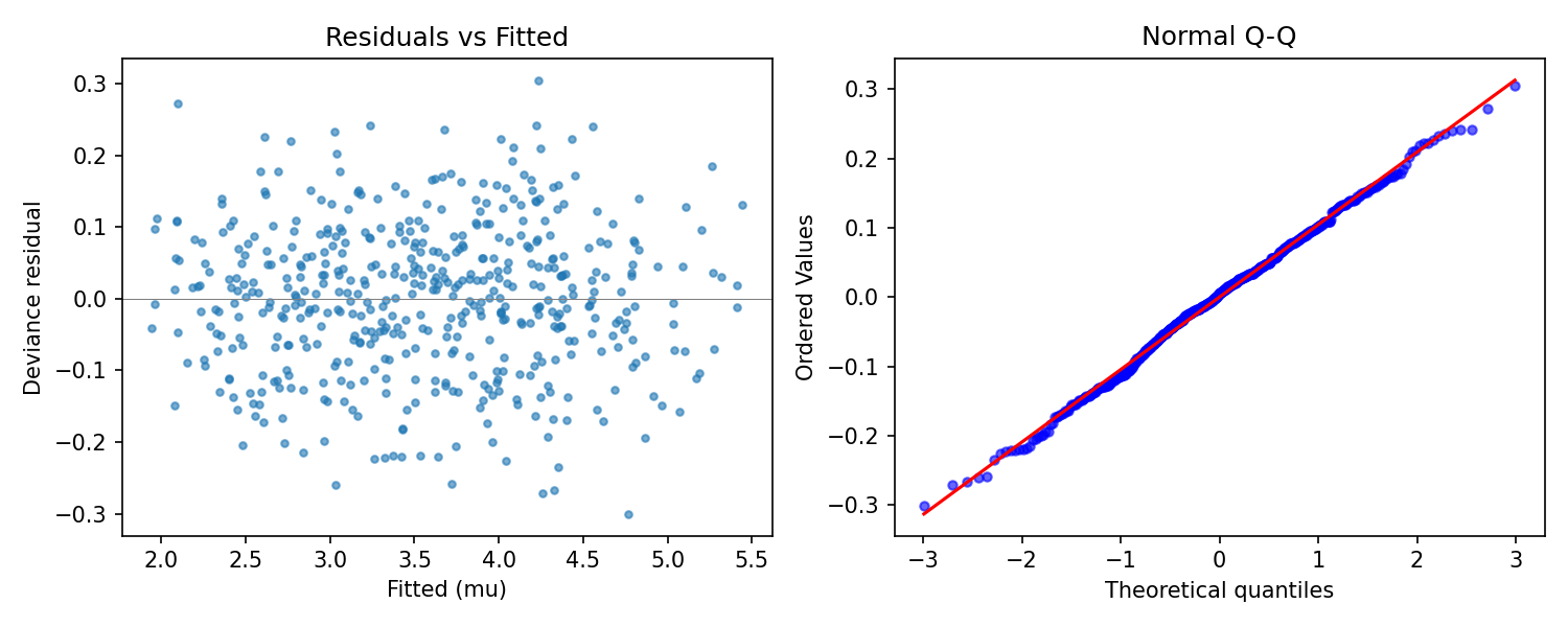
Output of mdl3.plot_residuals(): a featureless residual cloud on the left, and a Q-Q plot that tracks the reference line on the right. Both panels indicate the model has captured the systematic structure and that the Gaussian family is appropriate.

What you want to see:

• The left panel (residuals vs. \(\hat\mu\)) is a featureless cloud centered on zero. No trend, no funnel.

• The right panel (QQ against the standard normal) is a straight line. Heavy tails curl up at the top right and down at the bottom left; light tails do the opposite.

What you do not want to see:

• A clear curve in the left panel — the conditional mean is mis-specified somewhere (missing nonlinearity or wrong link).

• A funnel widening with \(\hat\mu\) — variance is mis-specified (consider a different family, or check whether the link is wrong).

• Pronounced QQ tails — the family’s tail is too thin or too thick; consider Huber loss for Gaussian-like data with outliers.

Residuals vs. a predictor

The fitted-value plot collapses every predictor onto \(\hat\mu\), which obscures which predictor a residual pattern is attached to. plot_residuals_vs_predictor() puts a chosen predictor on the x-axis instead.

For a predictor in the model, structure in the residuals indicates the feature is in the model in the wrong form — typically a linear term that should be a spline.

For a predictor not in the model, structure indicates the predictor carries signal the model is missing.

For example, plotting mdl3’s residuals against walkability — a predictor that is in the model, as a spline — should produce a featureless cloud, confirming that the spline has absorbed the walkability effect:

fig = mdl3.plot_residuals_vs_predictor(X['walkability'], name='walkability')

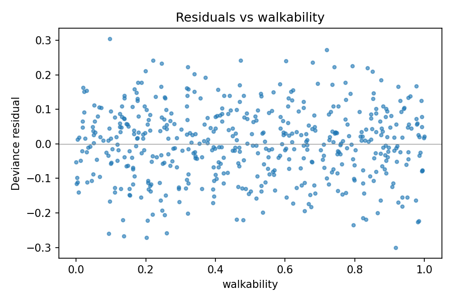
mdl3’s residuals against walkability: a featureless cloud, indicating the spline has captured the walkability effect. Compare with the analogous plot on mdl2 below, where the same predictor was missing.

A diagnosis-and-fix cycle

To make this concrete, consider an analyst who fits the simplest plausible model on the rent data and inspects it before reaching for features:

mdl1 = GAM(family='normal')
mdl1.add_feature('sqft', type='linear')
mdl1.fit(X, y)
mdl1.plot_residuals()

The QQ plot is roughly straight (the noise process is Gaussian by construction), but the left panel shows a wide vertical spread at every fitted value. The model’s \(\hat\phi \approx 0.135\) is more than ten times the true noise variance of \(0.01\), and the residuals reflect that. We have unmodelled signal somewhere; the question is where.

mdl1.plot_residuals_vs_predictor(X['neighborhood'], name='neighborhood')

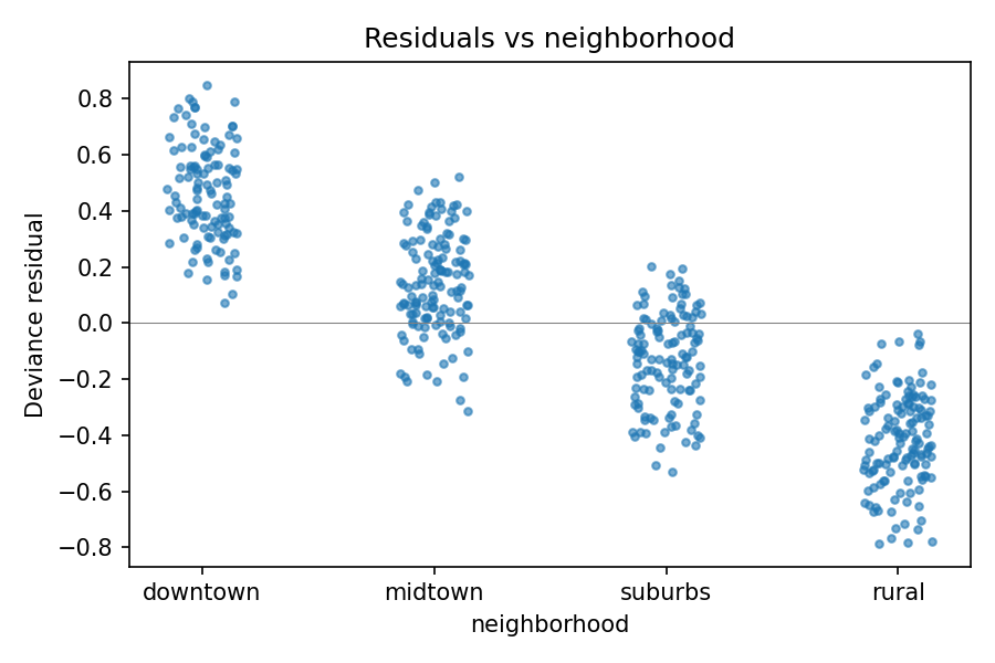
mdl1’s residuals stratify cleanly by neighborhood: the structure is the unmodelled neighborhood offset showing through.

Now the structure is unmissable: the residual cloud sits noticeably high for downtown, low for rural, with midtown and suburbs in between. That is the neighborhood offset showing through the residuals because the model has no way to absorb it. Adding neighborhood as a categorical feature is the obvious fix, and produces mdl2 from the getting-started guide.

After refitting, the same plot against walkability reveals the remaining structure:

mdl2.plot_residuals_vs_predictor(X['walkability'], name='walkability')

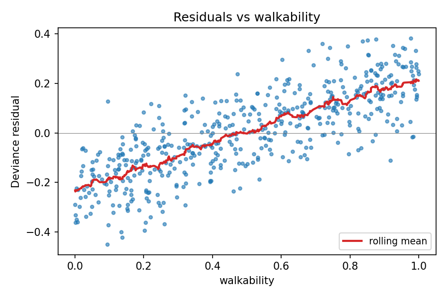
mdl2’s residuals against walkability: the rolling-mean overlay traces out a concave-increasing arc, the signature of an unmodelled nonlinear effect. The featureless version of this same plot for mdl3 appears above in Residuals vs. a predictor.

The residuals trace out a concave-increasing arc — exactly the shape of the true \(0.5 \cdot w^{0.7}\) effect that mdl2 ignores. Adding walkability as a spline feature (a linear term would not capture the curvature, and the residual plot would still show structure) gives mdl3. A final pass through plot_residuals() and plot_residuals_vs_predictor() for each predictor shows featureless residual clouds on every axis and a straight QQ plot — the diagnostics for mdl3 shown earlier are exactly that final pass. The model has captured the systematic structure.

Notice that residual diagnostics gave a much sharper verdict than the information-criteria comparison did. The AIC differences between mdl1, mdl2, and mdl3 were all in single digits — on AIC alone the case for the larger models is plausible but not crushing. The residual plots leave no doubt: mdl1 and mdl2 have unmodelled structure, mdl3 does not. In practice, use both: AIC / AICc to compare candidate models on a common footing, residual plots to check whether any of them is actually adequate.

A few practical notes

• Convergence first. A fit that did not converge will have meaningless residuals. Check that the primal / dual residual histories from fit() are below their tolerances before running diagnostics.

• Anscombe for QQ on small samples. The deviance residual is approximately standard normal in the limit, but on small samples its tails can be slightly off. Anscombe residuals are tuned to be more nearly normal in finite samples; switch with kind="anscombe" if the QQ plot’s tails look suspect.

• Predictor not on file. plot_residuals_vs_predictor() accepts any 1-D array of length n_obs, so you can plot residuals against a covariate that was never registered with add_feature(). This is the standard way to decide whether to add a new predictor before fitting it.

• Categorical x-axes work. Pass an object-dtype array (e.g., a column of strings) and the helper switches to a categorical x-axis automatically.