Reproducing the Paper#
“Randomization Inference for Matched Pairs with Binary Outcomes” [Wil26] develops its method around a single running example, returning to it in every section as the machinery grows: a composite null, the worst-case pattern, prediction sets, an ATE confidence set, and finally a sensitivity analysis. This guide reproduces each of those calculations with PairMatch, in the paper’s order, and cites the section, equation, figure, or table it reproduces. Every number quoted below is a doctest, executed each time the documentation is built, so the guide cannot drift from what the library computes.
The guide is also a tour of the library. Each step introduces the function that performs it, and the last section collects them into a single table.
The Running Example#
The paper’s example (§3) is a controlled experiment on \(S =
1{,}000\) pairs, with one unit in each pair selected at random for
treatment. Let \(S_{jk}\) count the pairs whose treated unit has
outcome \(j\) and whose control has outcome \(k\). In
\(S_{00} = 800\) pairs neither unit succeeded, in \(S_{11} =
100\) both did, in \(S_{10} = 70\) only the treated unit did, and in
\(S_{01} = 30\) only the control did. A
PairedOutcomeTable holds exactly these
four counts:
>>> from pair_match import PairedOutcomeTable
>>> table = PairedOutcomeTable(s00=800, s01=30, s10=70, s11=100)
>>> table.n_pairs
1000
>>> print(f"{table.treated_success_rate:.2f}, {table.control_success_rate:.2f}")
0.17, 0.13
The estimand is the attributable effect \(A_1\) [Ros02]: the number of successes among treated units caused by treatment, minus the number of successes treatment prevented. Its mirror \(A_0\) is the same quantity for the untreated. Both depend on which unit in each pair was treated, so they are random; their sum, \(A_1 + A_0 = 2S \cdot \mathrm{ATE}\) (equation 1), is not.
One Sharp Null#
A sharp null specifies the treatment effect for every unit, and so imputes the control outcome of every treated unit. McNemar’s test then counts, among the pairs discordant under those imputed control outcomes, the \(m_{+0}\) in which the treated unit is the success under control, and compares it with a \(\mathrm{Binom}(m_{+0} + m_{+1}, \tfrac{1}{2})\) reference distribution.
The paper’s first illustration (§3, Example) tests the pattern \(m_{+0} = 435\), \(m_{+1} = 65\), which is consistent with \(H_0: A_1 \leq 0\). The p-value is a single binomial tail:
>>> from scipy.stats import binom
>>> def p_greater(a, b):
...     """Pr{Binom(a + b, 1/2) >= a}, the right-tailed McNemar p-value."""
...     return binom.sf(a - 1, a + b, 0.5)
>>> print(f"{p_greater(435, 65):.3g}")
1.52e-68
McNemar’s test rejects this pattern overwhelmingly. But rejecting a composite null requires rejecting every pattern consistent with it: “to reject a composite hypothesis is to reject each and every way it may be true.” The consistent patterns fill the trapezoid of the paper’s Figure 1a, and there are thousands of them.
The Single Hardest Pattern#
Section 4 shows we need test only one. Lemma 1 says the p-value falls as \(m_{+0}\) grows with \(m_{+1}\) fixed, so on each horizontal slice of the trapezoid the hardest pattern to reject sits at its left edge. Along the \(m_{+1} = 65\) slice (the paper’s Figure 2), one step to the right of the example pattern roughly halves the p-value, and the supremum sits at \(m_{+0} = m_{+1} + \delta_0 = 105\), where \(\delta_0 = S_{10} - S_{01} - a_0 = 40\):
>>> print(f"{p_greater(436, 65):.3g}")
8.73e-69
>>> print(f"{p_greater(105, 65):.3g}")
0.00134
import numpy as np
import matplotlib.pyplot as plt
from scipy.stats import binom

m = np.arange(105, 871)
fig, ax = plt.subplots()
ax.semilogy(m, binom.sf(m - 1, m + 65, 0.5))
ax.axhline(0.05, color="tab:orange", linestyle="--", label=r"$\alpha = 0.05$")
ax.plot([435], [binom.sf(434, 500, 0.5)], "ko", label="example pattern")
ax.plot([105], [binom.sf(104, 170, 0.5)], "o", color="tab:red",
        label=r"supremum $(105,\ 1.3 \times 10^{-3})$")
ax.set_ylim(1e-200, 10)
ax.set_yticks([1, 1e-50, 1e-100, 1e-150, 1e-200])
ax.set_xlabel(r"$m_{+0}$ (with $m_{+1} = 65$)")
ax.set_ylabel(r"$p_{>}(m_{+0}, 65)$")
ax.legend()
fig.tight_layout()
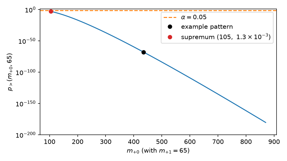
Figure 2 of [Wil26]: along the \(m_{+1} = 65\) slice, the p-value decreases in \(m_{+0}\), so the supremum over consistent patterns sits at the left endpoint \(m_{+0} = 105\).#
Lemma 1 therefore confines the search to the boundary \(m_{+0} = m_{+1} + \delta_0\). Lemma 2 says that when \(\delta_0 \geq 2\), the p-value increases along that boundary, so the hardest pattern lies at the largest \(m_{+1}\) the box constraints admit (the paper’s Figure 3):
import numpy as np
import matplotlib.pyplot as plt
from scipy.stats import binom

b = np.arange(0, 131)
fig, ax = plt.subplots()
ax.semilogy(b, binom.sf(b + 40 - 1, 2 * b + 40, 0.5))
ax.axhline(0.05, color="tab:orange", linestyle="--", label=r"$\alpha = 0.05$")
ax.plot([130], [binom.sf(169, 300, 0.5)], "ko", label=r"$(b^\star, p^\star)$")
ax.set_ylim(1e-12, 1)
ax.set_xlabel(r"$m_{+1}$ (boundary $m_{+0} = m_{+1} + 40$)")
ax.set_ylabel(r"$p_{>}(m_{+1} + 40, m_{+1})$")
ax.legend()
fig.tight_layout()
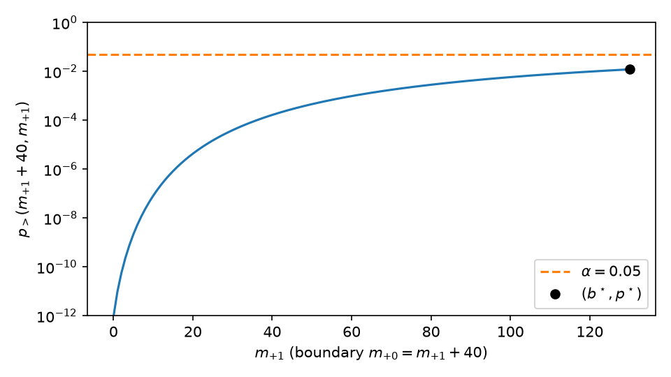
Figure 3 of [Wil26]: along the consistency boundary, the worst-case p-value increases in \(m_{+1}\) and peaks at the corner \((a^\star, b^\star) = (170, 130)\).#
Proposition 1 (equation 5) gives the corner in closed form,
which here is \(b^\star = \min(130, 830) = 130\) and \(a^\star
= 170\). Testing the composite null thus costs one binomial tail, and
this is exactly what worst_case_pvalue()
computes. The one-sided test of \(H_0: A_1 \leq 0\) matches the
paper’s \(0.0121\):
>>> from pair_match import worst_case_pvalue
>>> print(f"{p_greater(170, 130):.4f}")
0.0121
>>> p = worst_case_pvalue(table, target="ATT", null_value=0, alternative="greater")
>>> print(f"{p:.4f}")
0.0121
Since \(0.0121 < 0.05\), we reject \(H_0: A_1 \leq 0\). Note
that target="ATT" selects \(A_1\), the effect among the treated;
target="ATU" selects \(A_0\).
Prediction Sets#
Inverting the test gives a prediction set for \(A_1\) (§5). As the hypothesized \(a_0\) rises, \(\delta_0\) shrinks and the worst-case p-value grows; the lower endpoint \(L_\alpha\) is the smallest \(a_0\) the test fails to reject. The paper’s sweep shows the one-sided \(\alpha = 0.05\) test crossing between \(a_0 = 11\) and \(a_0 = 12\), and the mirror test crossing between \(66\) and \(67\):
>>> for a0 in (11, 12):
...     p = worst_case_pvalue(table, null_value=a0, alternative="greater")
...     print(a0, f"{p:.4f}")
11 0.0497
12 0.0557
>>> for a0 in (66, 67):
...     p = worst_case_pvalue(table, null_value=a0, alternative="less")
...     print(a0, f"{p:.4f}")
66 0.0510
67 0.0441
So \(L_{0.05} = 12\) and \(U_{0.05} = 66\), and their
intersection is the two-sided 90% prediction set \(A_1 \in [12,
66]\). attributable_effect_interval()
performs the whole binary search, in \(O(\log S)\) binomial tail
evaluations:
>>> from pair_match import attributable_effect_interval
>>> attributable_effect_interval(table, target="ATT", confidence=0.90)
(12, 66)
The Hodges-Lehmann point estimate (equation 8) is the observed surplus of treated-success discordant pairs, \(\hat{A} = S_{10} - S_{01} = 40\). The prediction set brackets it asymmetrically, with 28 units of room below and 26 above, because the binomial variance is larger at the lower crossing (\(n = a^\star + b^\star = 288\)) than at the upper (\(n = 234\)):
>>> table.hat_a
40
For large \(S\) the binary search admits a closed form (equations 9–11). On the top face of the constraint box the lower root is \(\delta_0^\star = 1 + \tfrac{1}{2}z^2 + z\sqrt{2(S_{01} + S_{11}) + 1 + \tfrac{1}{4}z^2}\); the mirror root for the upper endpoint flips the signs of the \(\tfrac{1}{2}z^2\) term and of the 1 inside the radical (Table 3). At \(z = z_{0.95}\), flooring each root lands on the binary-search values:
>>> import math
>>> from scipy.stats import norm
>>> z = norm.ppf(0.95)
>>> lower_root = 1 + z**2 / 2 + z * math.sqrt(2 * 130 + 1 + z**2 / 4)
>>> upper_root = 1 - z**2 / 2 + z * math.sqrt(2 * 130 - 1 + z**2 / 4)
>>> print(f"{lower_root:.2f} {upper_root:.2f}")
28.96 26.15
>>> 40 - math.floor(lower_root), 40 + math.floor(upper_root)
(12, 66)
(The paper quotes the upper root as \(26.16\), having rounded \(z_{0.95}\) to \(1.645\); the floor, and so the endpoint, is the same either way.)
PairMatch implements this approximation (the full Table 3, including the
right face and the self-consistency check between faces) as
method="normal". It agrees with the exact search here, as the paper
reports:
>>> attributable_effect_interval(table, target="ATT", confidence=0.90, method="normal")
(12, 66)
The same machinery gives the prediction set for \(A_0\), the net effect among the untreated, under the swapped box ceilings of equation 7. The paper reports \([11, 72]\) both exactly and from the Gaussian approximation:
>>> attributable_effect_interval(table, target="ATU", confidence=0.90)
(11, 72)
>>> attributable_effect_interval(table, target="ATU", confidence=0.90, method="normal")
(11, 72)
A Confidence Set for the ATE#
Section 6 combines the two prediction sets through equation 1. By the Bonferroni proposition of Rigdon and Hudgens [RH15], two \(1 - \alpha/2\) prediction sets \([L_1, U_1]\) for \(A_1\) and \([L_0, U_0]\) for \(A_0\) yield the \(1 - \alpha\) confidence set \([(L_1 + L_0)/2S,\, (U_1 + U_0)/2S]\) for the ATE. For a 90% set we therefore need 95% prediction sets:
>>> attributable_effect_interval(table, target="ATT", confidence=0.95)
(6, 70)
>>> attributable_effect_interval(table, target="ATU", confidence=0.95)
(5, 79)
>>> (6 + 5) / 2000, (70 + 79) / 2000
(0.0055, 0.0745)
expanded_confidence_interval()
runs the whole procedure (four binary searches); at gamma=1 it is
the randomization-based confidence set of §6:
>>> table.expanded_confidence_interval(alpha=0.10, gamma=1.0)
(0.0055, 0.0745)
The set brackets the point estimate \(\widehat{\mathrm{ATE}} =
(S_{10} - S_{01})/S = 0.040\) (equation 13) symmetrically, with half-width
\(0.0345\): the \(A_1\) set leans low about \(\hat{A} = 40\)
and the \(A_0\) set leans high, and the two asymmetries cancel in
the sum. analyze()
reports all of this at once, together with the worst-case p-value and
the sensitivity value we meet in the next section:
 >>> table.ate_hat
 0.04
 >>> print(table.analyze(alpha=0.10, target="ATE"))
 |    ATE |   Conf Int**   |   iSuccesses |  Conf Int**  |   p-Value* |      Γ• |
 |--------+----------------+--------------+--------------+------------+---------|
 | +4.00% | +0.55%, +7.45% |          +40 |   +6, +74    |    0.0484* | 1.03459 |
 *  An asterisk in the p-Value column indicates statistical significance at
    level 0.10, provided Γ≤1.
    p-Value is two-sided against the null hypothesis that iSuccesses = 0.
 ** Confidence intervals have coverage of at least 90%, provided Γ≤1.
The iSuccesses column is the same set on the count scale,
\(\mathrm{ATE} \cdot S = (A_1 + A_0)/2\).
The paper also gives a large-sample ATE interval in closed form (equation 12). It omits the continuity corrections, so its half-width, \(0.0339\), sits slightly inside the exact \(0.0345\):
>>> z = norm.ppf(1 - 0.10 / 4)
>>> half_width = z / 2000 * (
...     math.sqrt(2 * 130 + z**2 / 4) + math.sqrt(2 * 170 + z**2 / 4)
... )
>>> print(f"{half_width:.4f}")
0.0339
PairMatch’s method="normal" keeps the continuity corrections, and on
this table it reproduces the exact interval:
>>> table.expanded_confidence_interval(alpha=0.10, gamma=1.0, method="normal")
(0.0055, 0.0745)
Comparison With the Textbook McNemar Interval#
The textbook McNemar treatment [Fle13] models the four counts as a
multinomial sample and targets a difference of marginal success
probabilities. The two procedures share the point estimate but not the
width: the paper attributes a factor of about 2.1 to the null acting on
potential outcomes, to dropping monotonicity, and to the Bonferroni
combination. The Wald interval the paper quotes has half-width
\(z_{0.95}\sqrt{S_{01} + S_{10} - (S_{10} - S_{01})^2/S}\,/\,S\),
which is what mcnemar_ate_interval()
computes:
>>> z = norm.ppf(0.95)
>>> print(f"{z * math.sqrt(30 + 70 - 40**2 / 1000) / 1000:.4f}")
0.0163
>>> from pair_match import mcnemar_ate_interval
>>> lo, hi = mcnemar_ate_interval(table, confidence=0.90)
>>> print(f"{(hi - lo) / 2:.4f}")
0.0163
>>> print(f"{0.0339 / 0.0163:.1f}")
2.1
Sensitivity Analysis#
In an observational study, the treated unit of each pair need not have
been selected by a fair coin. Rosenbaum’s model ([Ros20], §3; the
paper’s §7, equation 14) lets
the within-pair selection probability \(\pi_s\) range over
\([1/(\Gamma + 1),\, \Gamma/(\Gamma + 1)]\), where \(\Gamma
\geq 1\) bounds the odds ratio of hidden bias. The worst-case corner
\((a^\star, b^\star)\) does not move; only the reference
distribution does, from \(\mathrm{Binom}(n, \tfrac{1}{2})\) to
\(\mathrm{Binom}(n, \Gamma/(\Gamma + 1))\). Every function above
therefore accepts a gamma argument.
Hodges-Lehmann Bounds#
Under the \(\Gamma\)-model the test statistic’s null expectation is
no longer known, so the Hodges-Lehmann point estimate becomes an
interval, with the closed-form endpoints of the paper’s Table 4. At
\(\Gamma = 1.25\) the non-monotonic bounds are
\(\mathrm{lb}_1 = S_{10} - \Gamma S_{01} - (\Gamma - 1) S_{11} =
7.5\) and \(\mathrm{ub}_1 = S_{10} - S_{01}/\Gamma + ((\Gamma -
1)/\Gamma) S_{11} = 66\) for \(A_1\), and (exchanging \(S_{00}\)
and \(S_{11}\)) \(\mathrm{lb}_0 = 6\) and \(\mathrm{ub}_0
= 82.5\) for \(A_0\). Combined through equation 1, the ATE point
estimate lies in \([(7.5 + 6)/2S,\, (66 + 82.5)/2S]\), which is
what sensitivity_analysis()
returns:
>>> gamma = 1.25
>>> lb1 = 70 - gamma * 30 - (gamma - 1) * 100
>>> ub1 = 70 - 30 / gamma + (gamma - 1) / gamma * 100
>>> lb0 = 70 / gamma - 30 - (gamma - 1) / gamma * 100
>>> ub0 = gamma * 70 - 30 + (gamma - 1) * 100
>>> lb1, ub1, lb0, ub0
(7.5, 66.0, 6.0, 82.5)
>>> lo, hi = table.sensitivity_analysis(gamma=1.25)
>>> print(f"{lo:.5f} {hi:.5f}")
0.00675 0.07425
>>> print(f"{(lb1 + lb0) / 2000:.5f} {(ub1 + ub0) / 2000:.5f}")
0.00675 0.07425
As \(\Gamma \to \infty\), the interval saturates at \(\hat{A}/2S \pm \tfrac{1}{2} = [-0.48, 0.52]\), the assumption-free partial identification region of Manski. The \(\Gamma\)-model interpolates between the randomization interval at \(\Gamma = 1\) and that region:
>>> lo, hi = table.sensitivity_analysis(gamma=1e9)
>>> print(f"{lo:.2f} {hi:.2f}")
-0.48 0.52
Expanded Confidence Intervals#
The sensitivity interval above carries hidden bias alone. The
expanded confidence interval also carries the randomness of the
assignment. The paper reports the large-sample version (Table 5 at
\(z = z_{1-\alpha/4}\)) widening and drifting to \([-0.029,
0.111]\) at \(\Gamma = 1.25\); PairMatch’s method="normal" gives
\([-57, 221]/2S\), which rounds to the paper’s endpoints, and the
exact inversion is one count narrower at each end:
>>> table.expanded_confidence_interval(alpha=0.10, gamma=1.25, method="normal")
(-0.0285, 0.1105)
>>> table.expanded_confidence_interval(alpha=0.10, gamma=1.25, method="exact")
(-0.028, 0.11)
The Sensitivity Value#
The sensitivity value \(\Gamma^\bullet\) [Zha19] is the largest \(\Gamma\) at which the study still rejects the null of no net effect. For the ATE at \(\alpha = 0.10\), the paper reports \(\Gamma^\bullet \approx 1.03\): an unmeasured confounder shifting the within-pair odds of treatment by as little as 3–4% could explain the effect.
>>> print(f"{table.gamma_star(alpha=0.10):.2f}")
1.03
>>> from pair_match import sensitivity_value
>>> print(f"{sensitivity_value(table, alpha=0.10, target='ATE'):.2f}")
1.03
plot_sensitivity()
draws the paper’s Figure 4: the point estimate, the sensitivity interval
nested inside the expanded confidence interval, and
\(\Gamma^\bullet\) where the expanded interval first reaches zero.
from pair_match import PairedOutcomeTable

table = PairedOutcomeTable(s00=800, s01=30, s10=70, s11=100)
data, ax = table.plot_sensitivity(
    target="ATE", alpha=0.10, gamma_max=1.5, legend_loc="upper left"
)
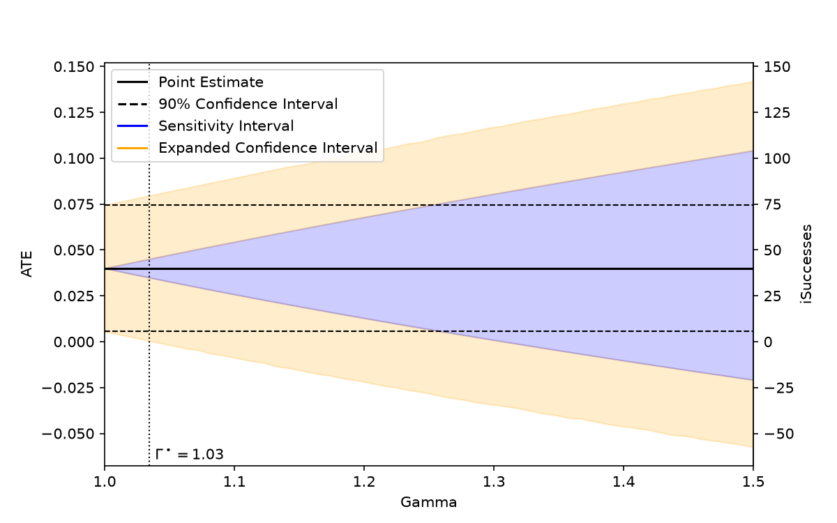
Figure 4 of [Wil26]: as \(\Gamma\) grows from 1, the sensitivity interval and the expanded 90% confidence interval widen around \(\widehat{\mathrm{ATE}} = 0.04\), and the expanded interval reaches zero at \(\Gamma^\bullet \approx 1.03\).#
Design Sensitivity#
\(\Gamma^\bullet\) mixes robustness to bias with ordinary sampling noise. The design sensitivity \(\tilde{\Gamma}\) removes the noise: it is the \(\Gamma\) beyond which no sample size could reject the null of no net effect. Without assuming monotonicity, and when the consistency line meets the top face of the box, \(\tilde{\Gamma} = (S_{10} + S_{11})/(S_{01} + S_{11}) = p_{1+}/p_{+1} = 1 + \tau/p_{+1}\). In the running example the control success rate is \(p_{+1} = 0.13\) and the effect is \(\tau = 0.04\), for a post-hoc design sensitivity of \(1.31\):
>>> from pair_match import design_sensitivity_binary
>>> print(f"{design_sensitivity_binary(baseline=0.13, ate=0.04):.2f}")
1.31
>>> print(f"{(70 + 100) / (30 + 100):.2f}")
1.31
A study of this effect size could never be made robust to hidden biases much beyond \(\Gamma = 1.31\), however many pairs it enrolled. The remedy is a better design, not a bigger sample. (As the paper warns, design sensitivity is most useful before a study is run; computing it post hoc carries the same caveats as post-hoc power analysis.)
Summary#
Every quantity in the paper’s running example is one PairMatch call:
Paper |
Value |
PairMatch |
|---|---|---|
§4, worst-case p-value, \(H_0: A_1 \leq 0\) |
0.0121 |
|
§5, 90% prediction set for \(A_1\) |
[12, 66] |
|
§5, 90% prediction set for \(A_0\) |
[11, 72] |
|
§5, equation 8, Hodges-Lehmann estimate |
40 |
|
§6, 90% ATE confidence set |
[0.0055, 0.0745] |
|
§7, Table 4, HL bounds at \(\Gamma = 1.25\) |
[0.00675, 0.07425] |
|
§7, expanded ATE interval at \(\Gamma = 1.25\) |
[−0.029, 0.111] |
|
§7, sensitivity value |
1.03 |
|
§7, Figure 4 |
|
|
§7, design sensitivity |
1.31 |
|
Only the lemma illustrations (Figures 2 and 3) and the paper’s
closed-form checks reach past the public API, to scipy.stats and
the formulas themselves; they verify the theory rather than use it.